Project: Planet Kaggle Competition - Satellite Image Analysis

The motivation

When machine learning finally evolved into a technology usable by the masses, it seemed like a super power. The whole idea of asking a computer to recognize something for you, and have it look through more data and with greater consistency than a person could do was game-changing.

But being new to the game, I needed to give this newfound superpower some exercise, so I went to Kaggle to find a competition to stretch my legs. Luckily there was a cool competition to classify satellite imagery in order to protect the rainforest. The idea was that the images were broken down into smaller tiles that were individually classified so that you could monitor how human developments and the rainforests were changing.

Random Forest with RGB Statistics

Luckily someone posted a quick getting started script that ran through a basic classifier using RGB statistics, which also included basic data import and formatting the submission. And while it originally called for the XGBClassifier, I substituted it out for a random forest model, since that was a part of the well-maintained sci-kit learn library. Plus random forest is my favorite machine learning algorithm being quick and usually getting a decent result =)

The RGB statistics was an interesting choice of feature using the mean, standard deviation, max, min, kurtosis, and skewness of each RGB channel across the image. Since these are aggregate statistics across the image, it removes the spatial information making the classifier essentially translationally invariant. Meaning white clouds could show up on any part of the image, and be classified as clouds. Of course, this also means white buildings could be confused as clouds or vice versa, since there is a substantial amount of information being lost.

But either way I gave it a shot, the random forest was set with 100 trees with all else being defaults, a random seed was set, the data was shuffled, and with 40479 samples a 80/10/10 split for training/validation/test sets. This was run at 5-times replicate while re-shuffling the dataset for each run. The aggregate results on the test set are reported below.

Individual F-Beta Scores for each run (beta=2 and average=sample):

0.83332, 0.83633, 0.84038, 0.83256, 0.83632

Combined F-Beta score: 0.83578

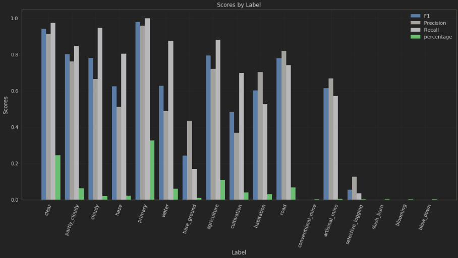
As we can see it does pretty well, even though it's essentially just looking at the the distribution of each RGB channel. However, it does particularly poorly on certain high frequency groups such as water and cultivation. To explain why it does poorly on water, it's best to look at some examples.

So sometimes brown means ground and sometimes brown means water. The reason why water is difficult is because we're dealing with very murky waters that isn't blue, and without additional information the classifier will have trouble telling the difference.

Random Forest with RGB Statistics + Edge/Line Statistics

Now there is a characteristic of water that we can exploit, the surface tends to be completely flat and uniform. This might already be picked up somewhat by the kurtosis and standard deviation, although it is an aggregate statistic over just three channels for the entire image. This sharp peak could be completely muddled by other colors. So if we can provide more information from another perspective, it might help the classifier differentiate and overall perform better.

So being flat and uniform, this also means there shouldn't be any edges on the surface of the water. So for fun, practice, and to use it, I implemented a quick website with a custom API to provide a graphical interface to quickly test different settings on some image processing algorithms that will return edges, lines, and corners. If you want to check it out, here's the link.

In addition, habitation and roads will often times have straight lines, while habitation should also be rich in corners.

However, we are not tuning the settings for each image, it's only one setting for the entire dataset. Even though one could make a machine learning algorithm to set the image processor settings based on the image, we're not going to do that at the moment. And as we can see below, due to these global settings sometimes they don't work out very well.

However, we'll still experiment with these additional features. Also to be more specific, we'll be using the sums of each edge/line/corner feature. For example for edges, there'll be an array of all the pixels on the image, and that pixel will either have a positive value representing the edge or zero, then we sum up the values across the array. These sums are appended to the existing RGB statistics training set. Also luckily because the random forest is a decision tree, we don't need to worry about scaling these values.

Model was setup with same settings as before with the only difference being the additional edge/line/corner statistics. (The random forest set with 100 trees with all else being defaults, a random seed was set, the data was shuffled, and with 40479 samples a 80/10/10 split for training/validation/test sets. This was run at 5-times replicate while re-shuffling the dataset for each run. The aggregate results on the test set are reported below.)

Individual F-Beta Scores for each run (beta=2 and average=sample):

0.83623, 0.84224, 0.84732, 0.8406, 0.84303

Combined F-Beta score: 0.84189

Looks like we were able to get a small improvement on average, and only by running randomized replicates we can have some confidence in detecting these small improvements, which is really what separates the top score from the rest. Luckily assuming a normal distribution and unequal variance, the two-sample T-test where the null hypothesis is that the two methods yield identical results on average is rejected with a one-sided p-value of 0.01453.

Submitting the results of this model run on the competition test set resulted in a F_beta score of 0.83062.

If we wanted to further pursue this direction, we would likely be able to get an even better result if we were to automate the exploration of the image processor hyperparameters. However, there are other things I want to try first.

Deep Neural Networks on the cloud

So specifically I want to try out deep convolutional neural networks, and training these models is a lot faster with a GPU. Unfortunately my computer is a Mac with a woefully underpowered GPU, so I decided to spin up a EC2 instance on Amazon Web Services.

I didn't really trust any of the AMIs that were out there that had this stuff installed (Keras, Tensorflow, Anaconda, CUDA, and cuDNN), so I setup the build process myself writing down the different bash commands I needed to get it done. Here are my notes in case anyone else is interested: 

# Setup EC2 instance

sudo apt-get update
sudo apt install gcc
sudo apt-get install linux-headers-$(uname -r)

# Go to https://www.continuum.io/downloads and set your installation parameters. Then modify the wget and bash to download and run the installation.

wget https://repo.continuum.io/archive/Anaconda3-4.3.1-Linux-x86_64.sh
bash Anaconda3-4.3.1-Linux-x86_64.sh
export PATH=/home/ubuntu/anaconda3/bin:$PATH

# When installing CUDA and cuDNN, google search 'Tensorflow gpu' and double check which versions to install. For instance, the tensorflow-gpu version as of writing used CUDA 8.0 and cuDNN 5.1, even though cuDNN 6.0 is the latest available. So double check
# Go to https://developer.nvidia.com/cuda-downloads and set your installation parameters. Then modify the wget and dpkg to download and run the installation

wget http://developer.download.nvidia.com/compute/cuda/repos/ubuntu1404/x86_64/cuda-repo-ubuntu1404_8.0.61-1_amd64.deb
sudo dpkg -i cuda-repo-ubuntu1404_8.0.61-1_amd64.deb
sudo apt-get update
sudo apt-get install cuda

# NOTE: Their installation guide as of writing has a typo when setting the PATH, it isn't cuda-8.0.61, the folder is just cuda-8.0

export PATH=/usr/local/cuda-8.0/bin${PATH:+:${PATH}}
export LD_LIBRARY_PATH=/usr/local/cuda-8.0/lib64\
 ${LD_LIBRARY_PATH:+:${LD_LIBRARY_PATH}}

# Download files from https://developer.nvidia.com/rdp/cudnn-download (you'll need to sign up/sign in) and copy to computer/server.

sudo dpkg -i libcudnn5_5.1.10-1+cuda8.0_amd64.deb
pip install tensorflow-gpu
pip install keras

And at this point you can just pip install whatever else you need. Currently a p2.xlarge holding a nvidia K80 is about $0.90 per hour, so it isn't too expensive, but after it all adds up it isn't cheap either.

Deep neural network

Designing the architecture of a neural network has often been considered a form of black magic. You kinda have an idea of what you're doing but it's difficult to figure out exactly how many layers, how many neurons per layer, etc without some form of trial and error.

However, there are certain high level ideas about the architecture that are very successful. Probably one of the most well known and popular one is fine-tuning a pre-trained network.

So what happens is you take a neural network that's been already carefully architected and trained on thousands of data points. And this output of this neural network is feed into a final output layer that's trained on the labels your trying to classify.

I personally used the Xception pretrained network that was already included in Keras, which was trained on the ImageNet dataset. So the output of this network is a list of probabilities of a particular classification like 13% chance of a watermelon, 68% chance of a ball, and etc. Now this output is used as an input for the final output layer to classify satellites image tiles as cloudy, river, habitation, etc.

But why does this work? Why would a neural network trained on mostly things that aren't our labels help? It's because some of those things look like the labels we care about. For instance, to the pretrained model a river can look like a river, but also a snake or garden hose. These other labels will have a higher output value, which our final output layer will learn how to synthesize together to produce a probability for our labels.

And since these pre-trained networks are so accurate and robust, we only need one layer with as many neurons as we have labels. So it's pretty straightforward.

Submitting the results of this model run on the competition test set resulted in a F_beta score of 0.88813. A huge nearly 6% improvement!

Feature Design

Now there's this thing in machine learning called feature design. And the idea is that you want to make it as easy as possible for your machine learning algorithm to do it's job. So if you can preprocess the input so that it highlights the important information you want your machine learning algorithm to consider, it will perform better.

So what I did was combine the pre-trained Xception neural network output with the image RGB statistics into the final output layer. This was because I noticed the image RGB statistics performed better in certain areas compared to the fine tuned pre-trained network alone, particularly with clear, partly_cloudy, cloudy, and haze labels. This makes some sense, because it's essentially how white is the image. Also these labels were assigned to a large percentage of the images, so even a marginal improvement here can have a noticeable impact on overall accuracy.

Submitting the results of this model run on the competition test set resulted in a F_beta score of 0.90007 in position 91 out of 253 as of writing.

Conclusion

After hitting the 0.9 threshold, I was pretty much satisfied with the result, and stopped working on it. I essentially got a A-!

This was approximately half way through the competition time. Eventually I went back and took a look at the final winning score, it was 0.93317. Not too far off from what I got.

It also appeared that the highest scoring competitors had a common optimization of trying out various pre-trained networks to fine-tune and picking the best result. I can see how that can definitely help move the score around 1 or 2 percentage points.

Overall, it was extremely fun and I learned a lot. It's super cool to try to build something to help save the Amazon rainforest, and I'm definitely looking for the free time to dip my toes back into machine learning again!